Deep Learning for Computer Vision
Train Neural Network
One time setup
Activation functions
Sigmoid: \(\sigma(x)=1/(1+e^{-x})\)
- Squashes numbers to range \([0,1]\)
- problems:
- Saturated neurons "kill" the gradients
- Sigmoid outputs are not zero-centered
- exp() is a bit compute expensive
Tanh
- Squashes numbers to range \([-1,1]\)
- zero centered(nice)
- still kill gradients when saturated
ReLU: \(f(x)=max(0,x)\)
- Does not saturate in positive region
- Very computationally efficient
- COnverges much faster than sigmoid/tanh in practice
- Problems:
- Not zero-centered output
- When x < 0, the gradient will also be zero, which may cause it never update.
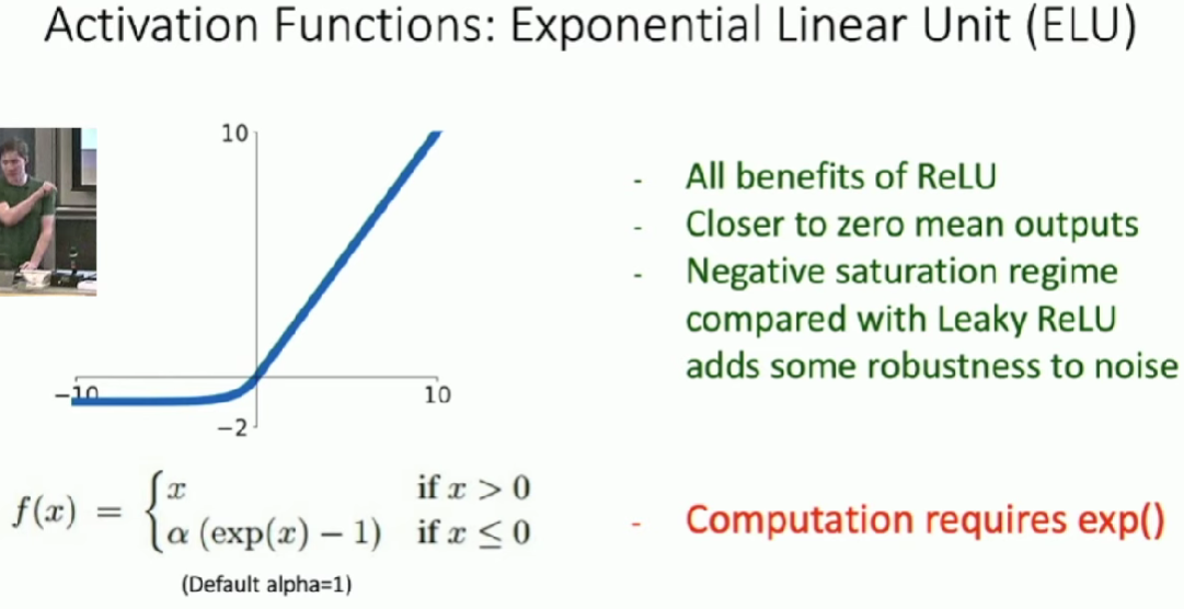
Leaky ReLU: \(f(x)=max(0.01x,x)\)
- Does not saturate
- Very computationally efficient
- COnverges much faster than sigmoid/tanh in practice
- will not "die" like ReLU
- We can introduce learnable parameter \(\alpha\), which is call PReLU(Parametric Rectifier): \(f(x)=max(\alpha x,x)\)
Data Preprocessing
- Subtract the mean image(AlexNet)
- Subtract per-channel mean(VGGNet)
- Subtract per-channel mean and divide by per-channel std(ResNet)
- Others
- PCA: data has diagonal covariance matrix
- whitening: covariance matrix is the identity matrix
Weight Initialization
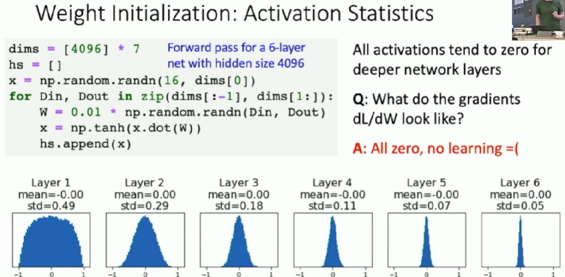
Q: What happens if we initialize all \(W=0, b=0\)?
A: All outputs are zero and weights will never update.
Small random values
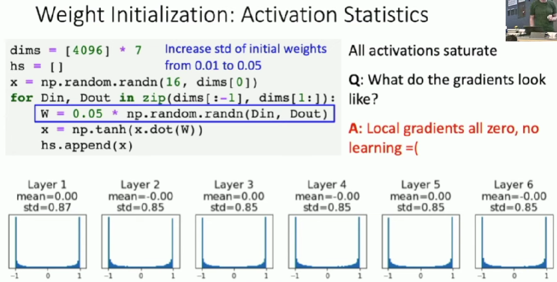
Big random values
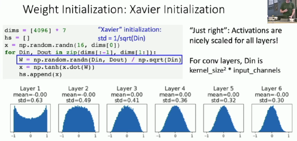
Xavier Initialization
- Derivation: Varience of output = Variance of input
Unfortunately, this initialization tends to be bad when we use ReLU as activation function.
Kaiming / MSRA Initialization * ReLU correction: std = sqrt(2 / Din)
"Just right" - activations nicely scaled for all layers.
Not do well in Residual Networks.
If we initialize with MSRA: then \(Var(F(x))=Var(x)\). But then \(Var(F(x)+x)>Var(x)\) - variance grows with each block!
- Solution: Initialize first conv with MSRA, initialize second conv to zero. Then \(Var(x+F(x))=Var(x)\)
Regularization
In common use: L2 regularization, L1 regularization ...
Dropout In each forward pass, randomly set some neurons to zero. Probability of dropping is a hyperparameter. 0.5 is common
Forces the network to have a redundant representation. Prevents co-adaptation of features.
Another interpretation: Dropout is training a large ensemble of models (that share parameters). Each binary mask is one model
- Test Time: We need to take another way to compute output when testing or our output will be random.
- We want to "average out" the randomness at test-time. That is, multiply the result without dropout by dropout probobility.
Inverted Dropout Drop and scale layer during training,
Data Augmentation
Tranform input training image before feeding it into the network. Horizontal flips is one example. This augments the amount of data and keep their label unchanged.
Random Crops and Scales
-
Training: sample random crops / scales
- Pick random L in range [256, 480]
- Resize training image, short side = L
- Sample random 224 x 224 patch
-
Testing: average a fixed set of crops
- Resize image at 5 scales: {224, 256, 384, 480, 640}
- For each size, use 10 224 x 224 crops: 4 corners + center, + flips
Training Dynamics
Learning rate schedules
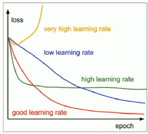
We can Start with large learning rate and decay over time.
Step Schedule
Step: Reduce learning rate at a few fixed points.
E.g. for ResNets, multiply LR by 0.1 after epochs 30, 60, and 90.
- Problem: introduce additional hyperparameters we have to tune.
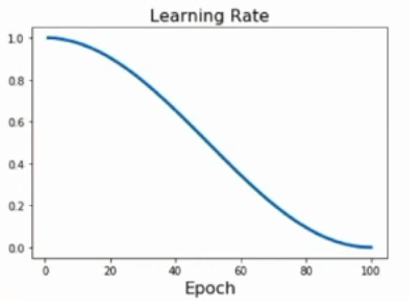
Cosine Schedule: \(\alpha_{t}=\frac{1}{2}\alpha_{0}(1+cos(t\pi /T))\)
Linear Schedule: \(\alpha_{t}=\alpha_{0}(1-t/T)\)
Inverse Sqrt: \(\alpha_{t}=\alpha_{0}/\sqrt{t}\)
Constant: \(\alpha_{t}=\alpha_{0}\)
- Early Stopping: Stop training the model when accuracy on the validation set decreases. Or train for a long time, but always keep track of the model snapshot that worked best on val. Always a good idea to do this!
hyperparameter optimization
Grid Search
Choose several values for each hyperparameter(Often space choices log-linearly).
Example:
Weight decay: [1x10⁻⁴, 1x10⁻³, 1x10⁻², 1x10⁻¹], Learning rate: [1x10⁻⁴, 1x10⁻³, 1x10⁻², 1x10⁻¹]
Evaluate all possible choices on this hyperparameter grid.
Random Search
Randomly choose several values for each hyperparameter in a given range(Often space choices log-linearly)
Example:
Weight decay: log-uniform on [1x10⁻⁴, 1x10⁻¹], Learning rate: log-uniform on [1x10⁻⁴, 1x10⁻¹]
- Jump out of the grid and may have a better performance when some parameters are not important.
Choosing hyperparameters:
Step 1: Check initial loss
Turn off weight decay, sanity check loss at initialization
Step 2: Overfit a small sample
Try to train to 100% training accuracy on a small sample of training data (~5-10 minibatches); fiddle with architecture, learning rate, weight initialization. Turn off regularization.
Loss not going down? LR too low, bad initialization
Loss explodes to Inf or NaN? LR too high, bad initialization
Step 3: Find LR that makes loss go down
Use the architecture from the previous step, use all training data, turn on small weight decay, find a learning rate that makes the loss drop significantly within ~100 iterations
Step 4: Coarse grid, train for ~1-5 epochs
Step 5: Refine grid, train longer
Step 6: Look at loss curves
Step 7: GOTO step 5
After training
Model ensembles
-
Train multiple independent models
-
At test time average their results
Transfer learning
-
Train on Imagenet
-
Use CNN as a feature extractor. Remove those fully connected layers in the last and freeze other layers.
-
Bigger dataset: Fine-Tuning
Reinitialize those last layer to new layers and continue training CNN for new task.
Some tricks:
-
Train with feature extraction first before fine-tuning
-
Lower the learning rate: use ~1/10 of LR used in original training
-
Sometimes freeze lower layers to save computation
Large-batch training
How to scale up on data-parallel training on K GPUs?
Goal: Train for same number of epochs, but use larger minibatches. We want model to train K times faster
Single-GPU model: batch size N, learning rate \(\alpha\)
K-GPU model: batch size KN, learning rate \(K\alpha\)
