Deep Learning for Computer Vision
Optimization
- goal: find \(w^{*}=argmin_{w}L(w)\)
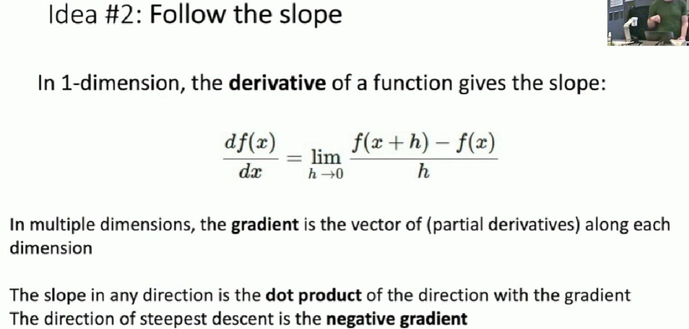
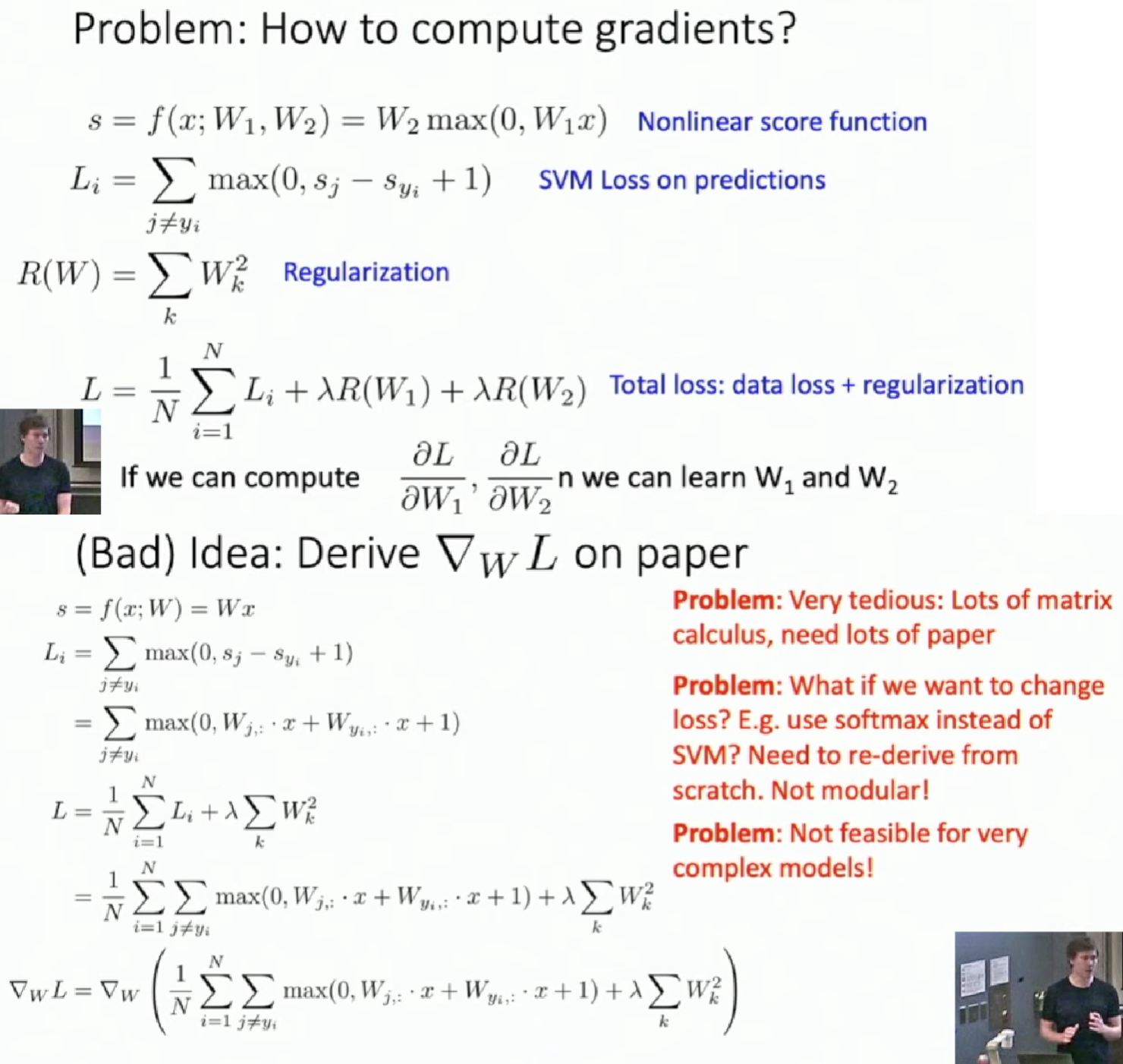
How to evaluate gradient?
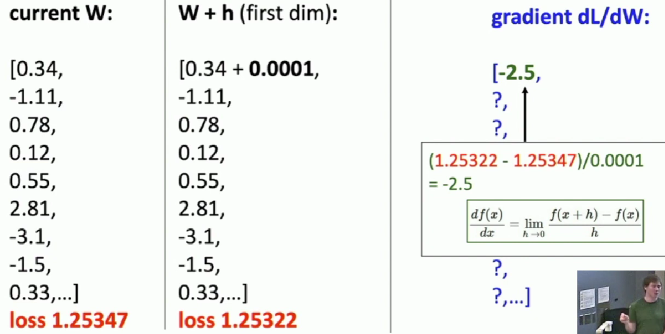
- Numeric gradient
- We can approximate the gradient by defination. Increasing one slot of the weight matrix by a small step and recompute loss function. Use the defination of derivative to get a approximation of gradient.
- Takes lots of time and not accurate.
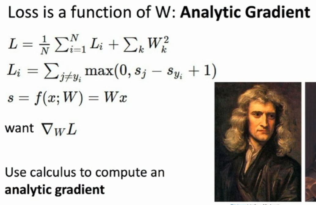
- Analytic gradient
- exact, fast, error-prone
- In practice, always use analytic gradient, but check implementation with numerical gradienet. This is called a gradient check
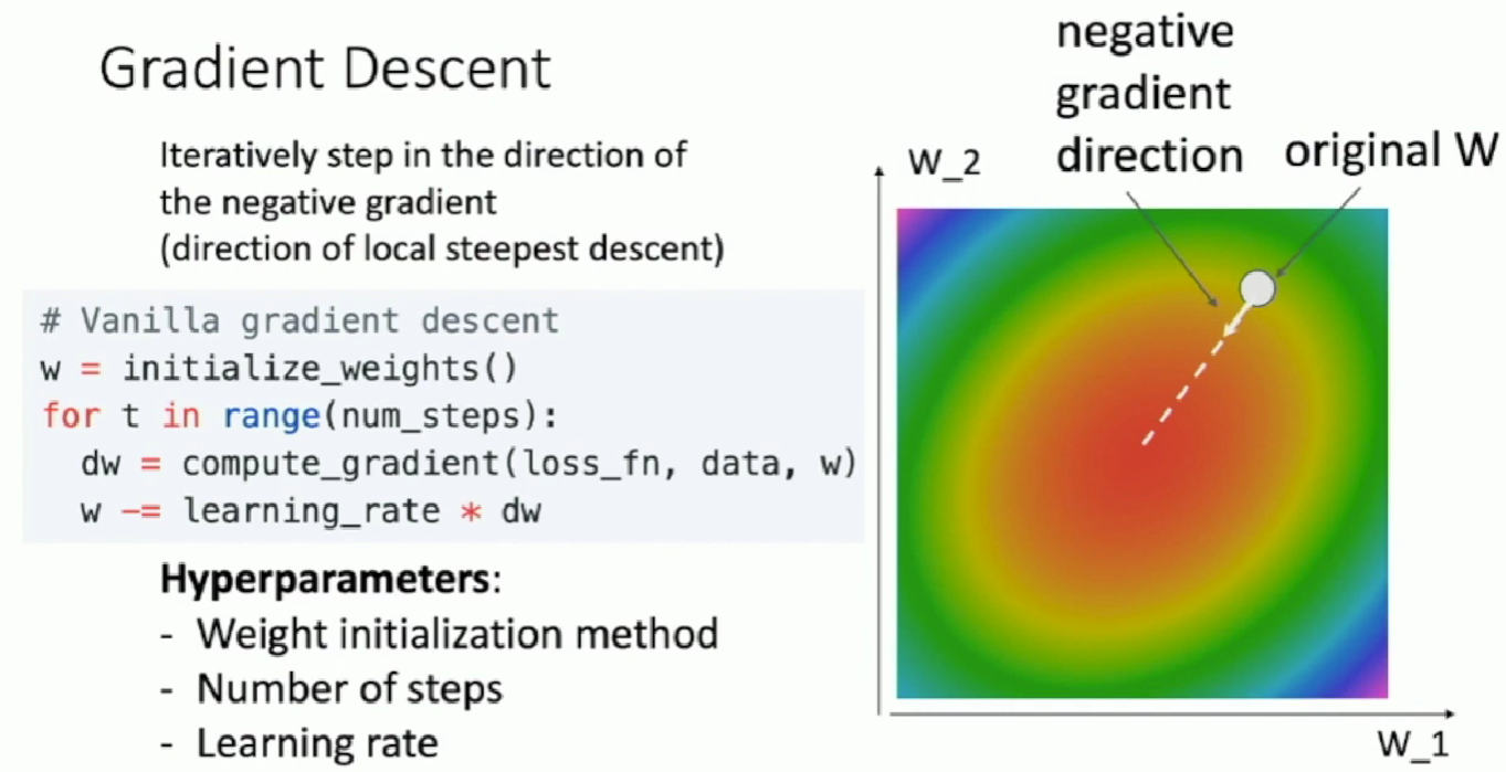
Gradient Descent
Stochastic Gradient Descend
- We don't use the full training data but some small subsamples of it to approximate loss function and gradient, for computing on the whole set is expansive. These small subsamples are called minibatches
- SGD + Momentum may overshoot in the bottom for its historical speed and will come back.
-
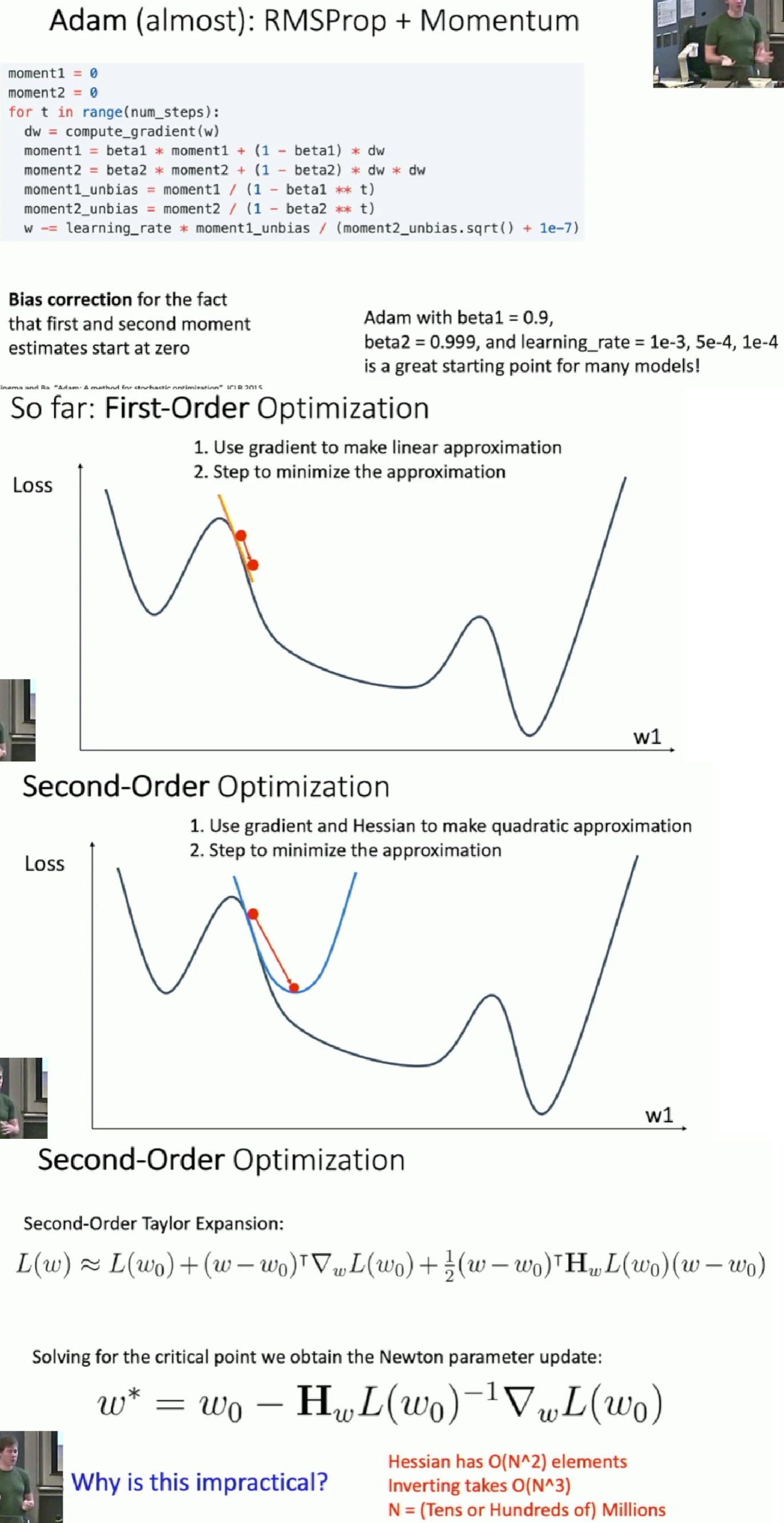
Progress along "steep" direction is damped. Progress along "flat" directions is accelerated.
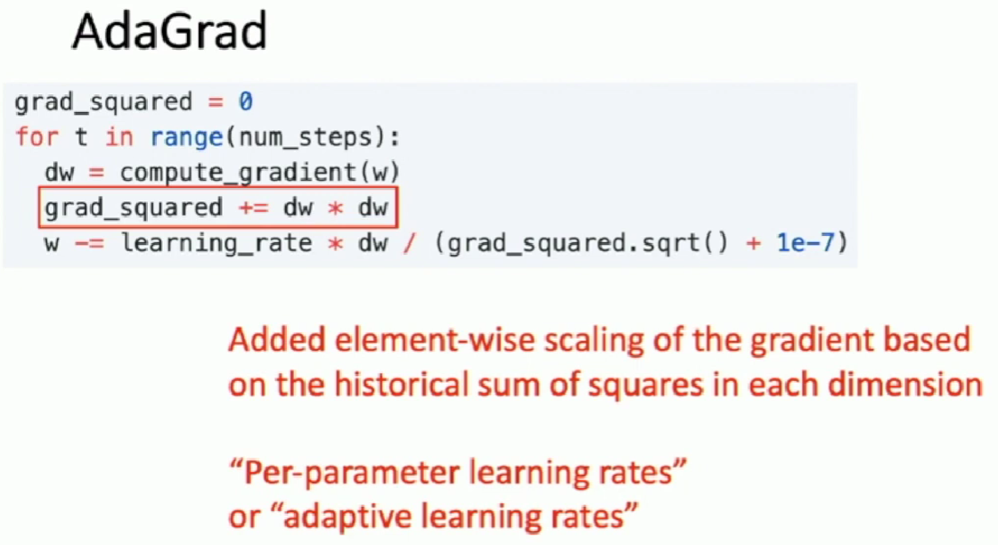
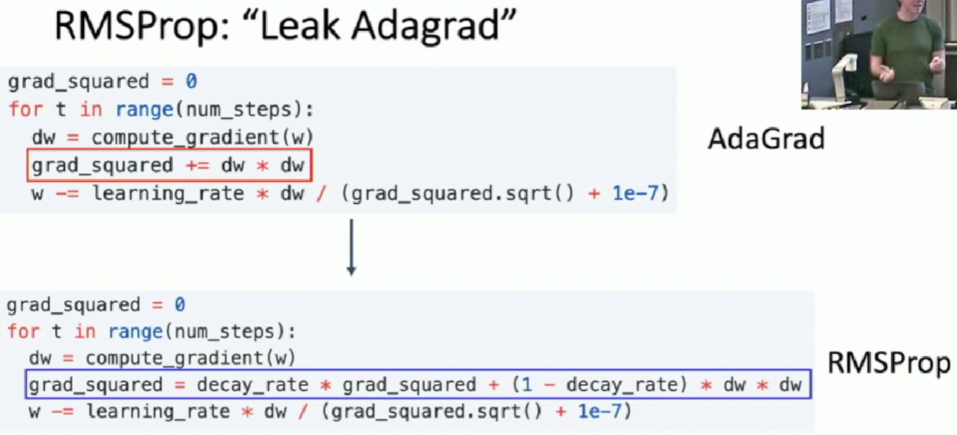
-
The learning rate will continuely decay since
grad_squaredgets larger and larger.
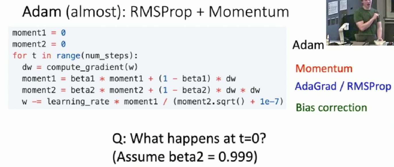
- We initialize
moment2as 0 and if we takebeta2closely to 0, themoment2will also close to 0, which may make our first gradient step very large. This could cause bad results.
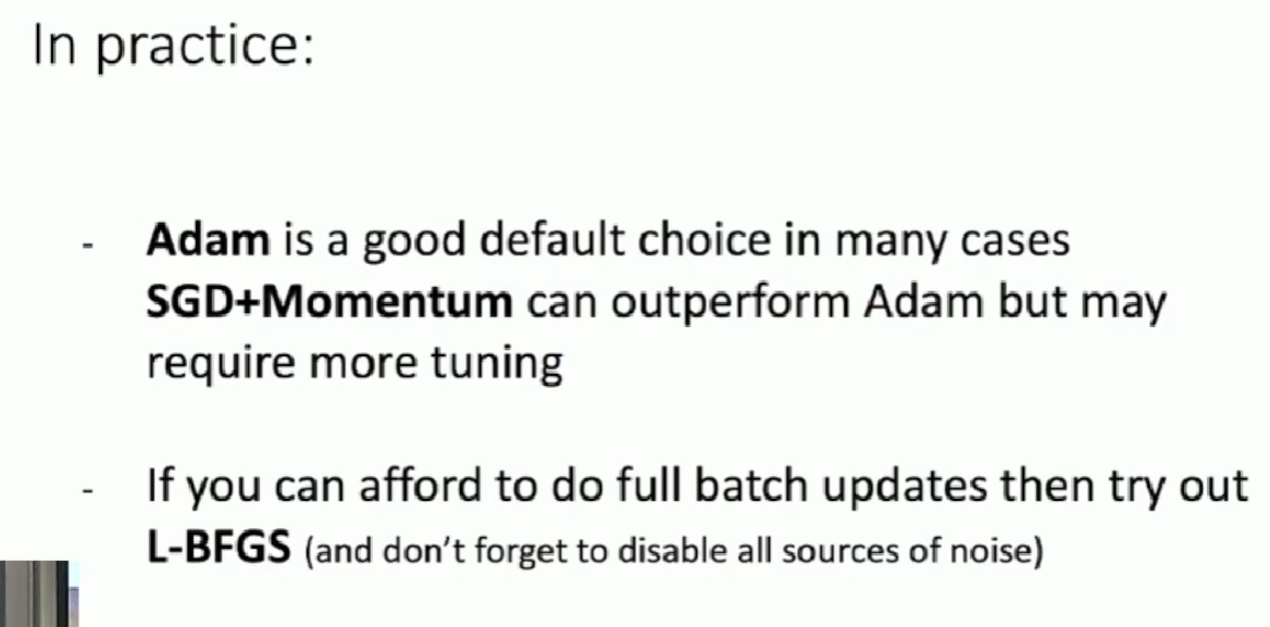
- Second-order optimization is better to use in low dimension.
Neural Network
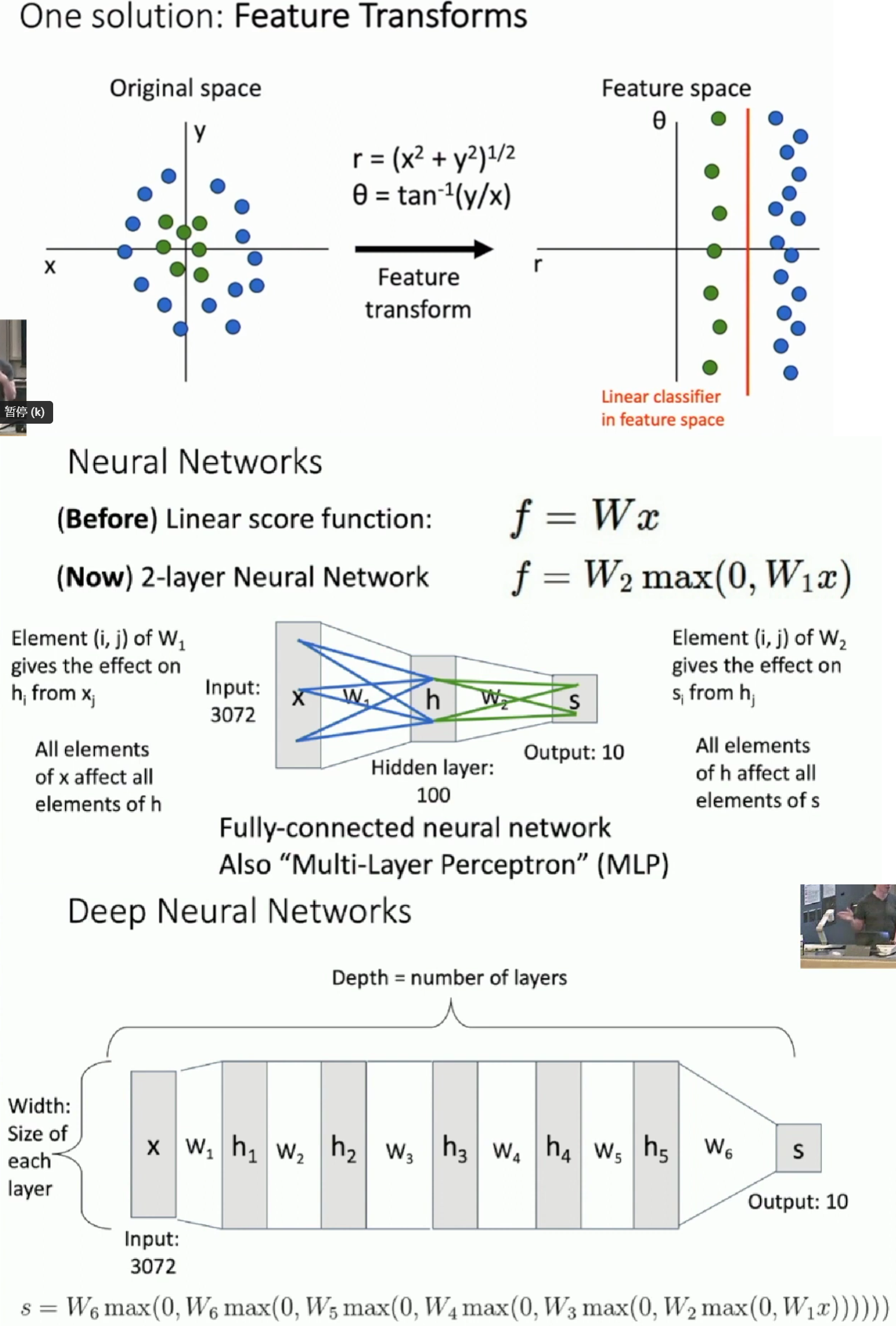
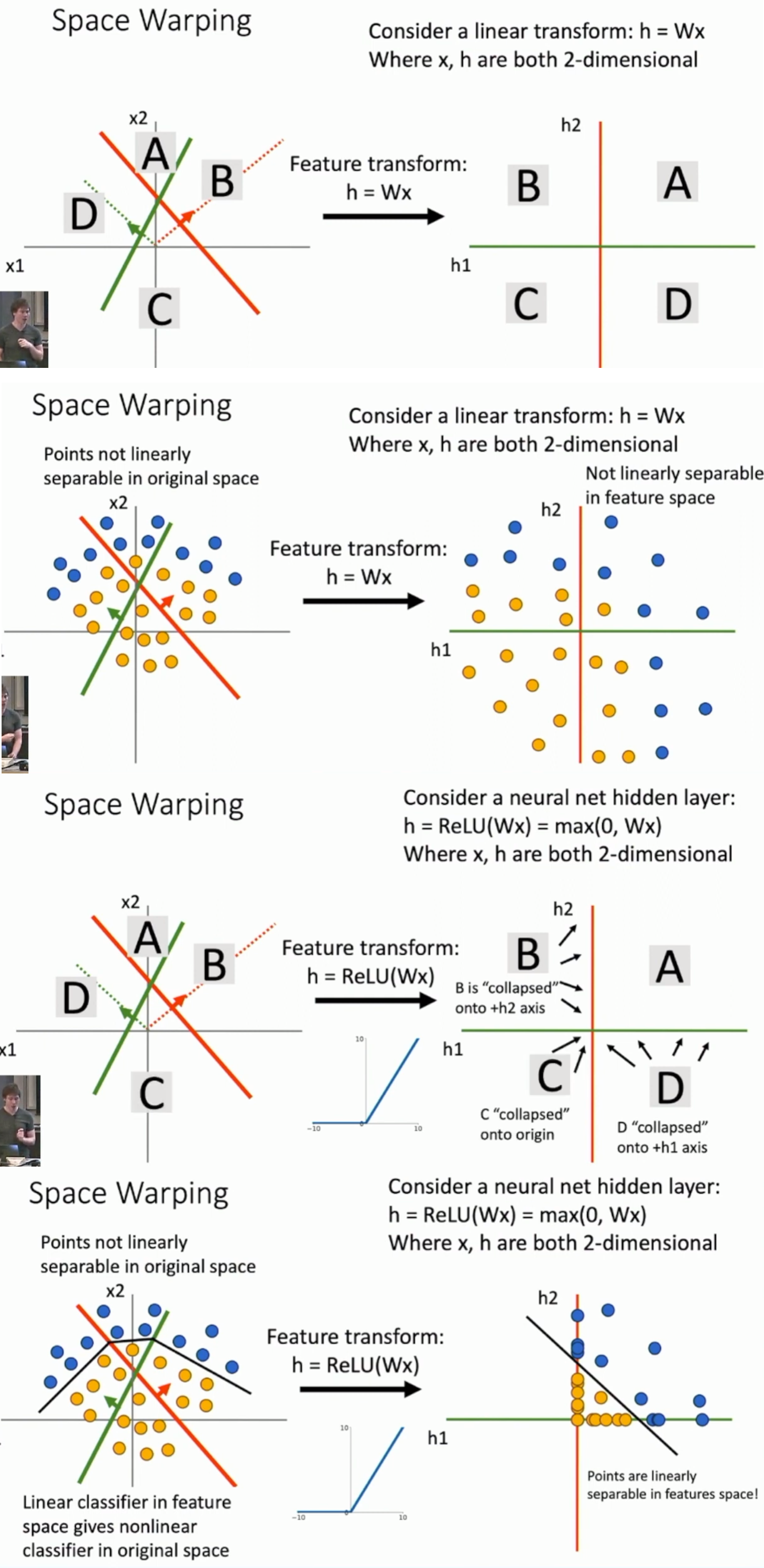
To solve the limitation of linear classifier, we can apply feature transformation.
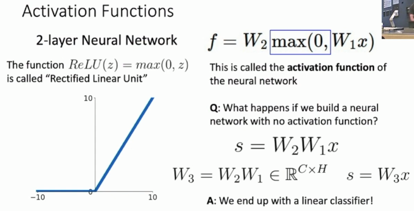
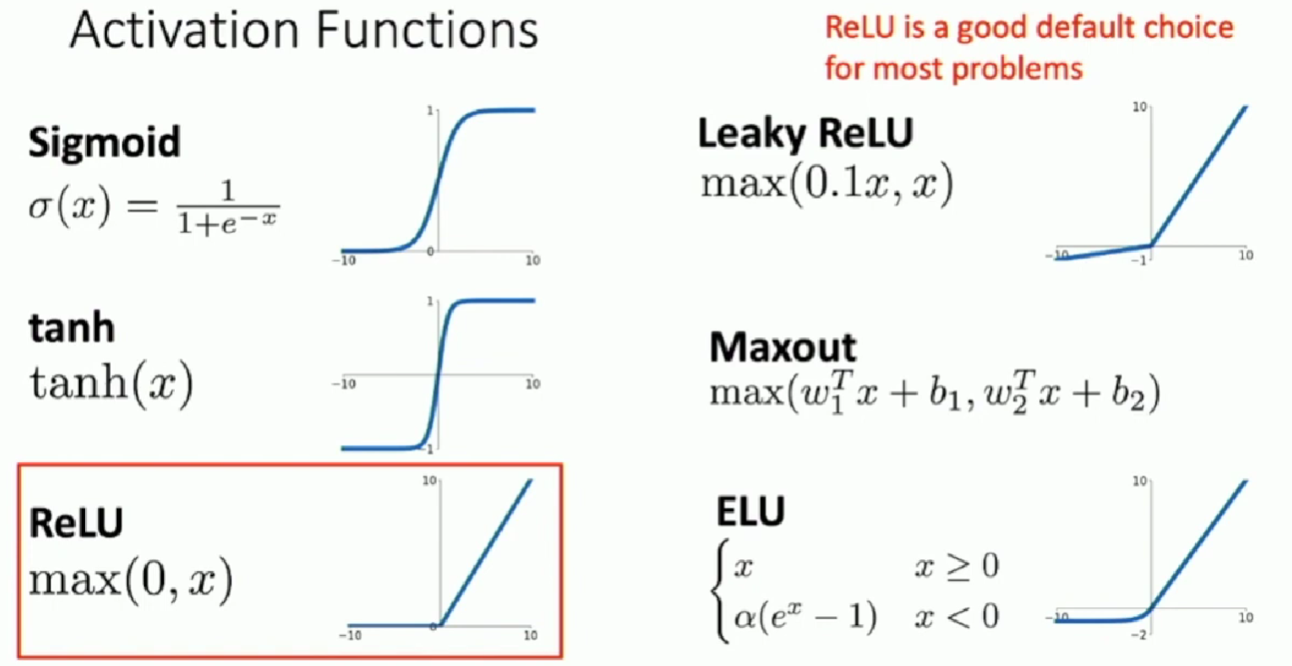
Activation function
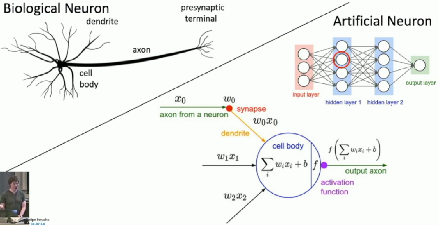
Neuron
Space Warping
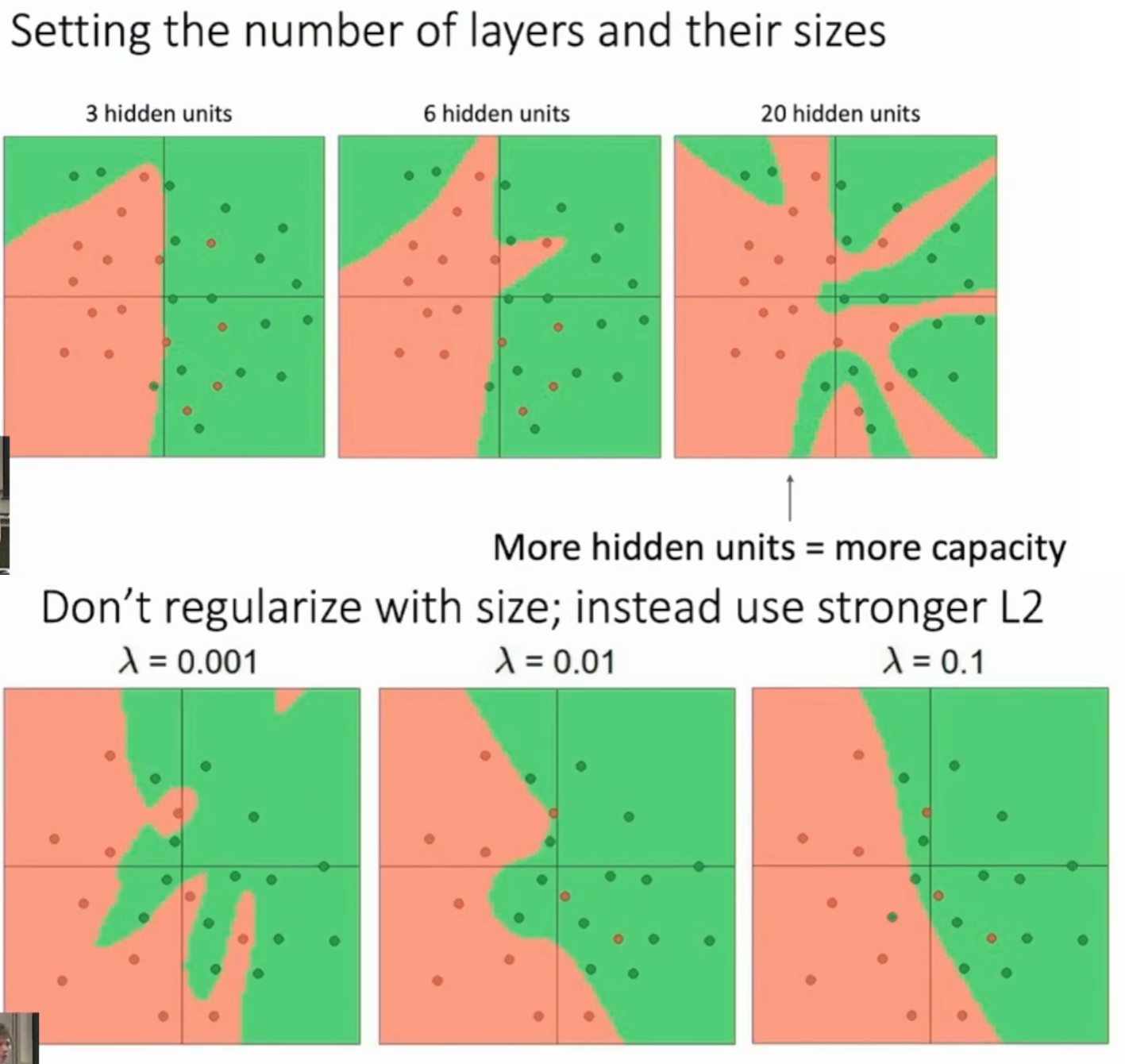
The more the layer, the more complex the model is. Try to adjust regularization parameter to solve it.
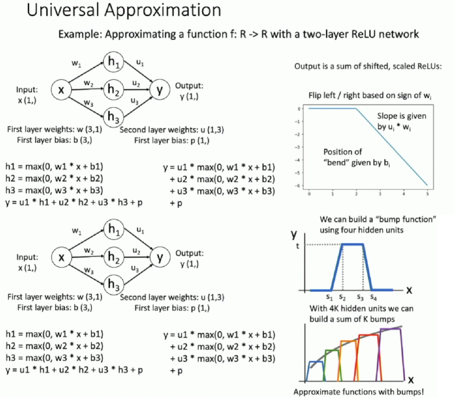
Universal Approximation
A two layer neural network can approximate any function. But it may need a large size to get high fidelity.
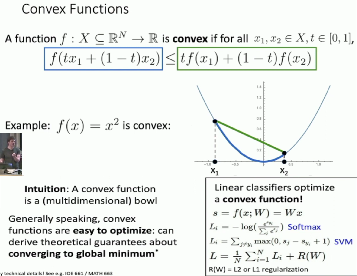
Convex Functions
Taking any two points in the input, the secant line will always lie above the function between that two points.
However, most neural networks need nonconvex optimization
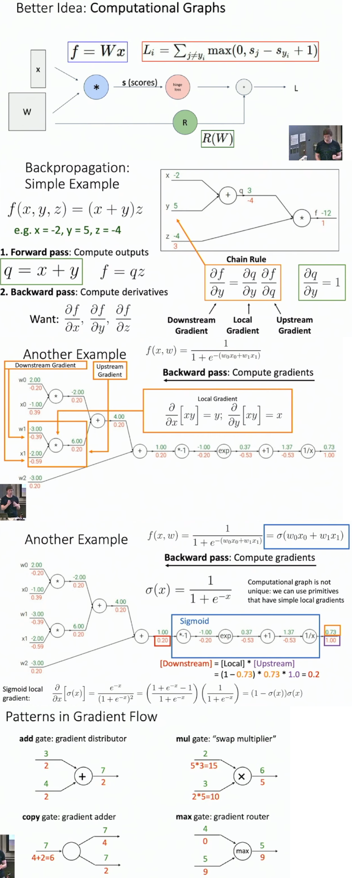
Backpropagation
Computation Graph
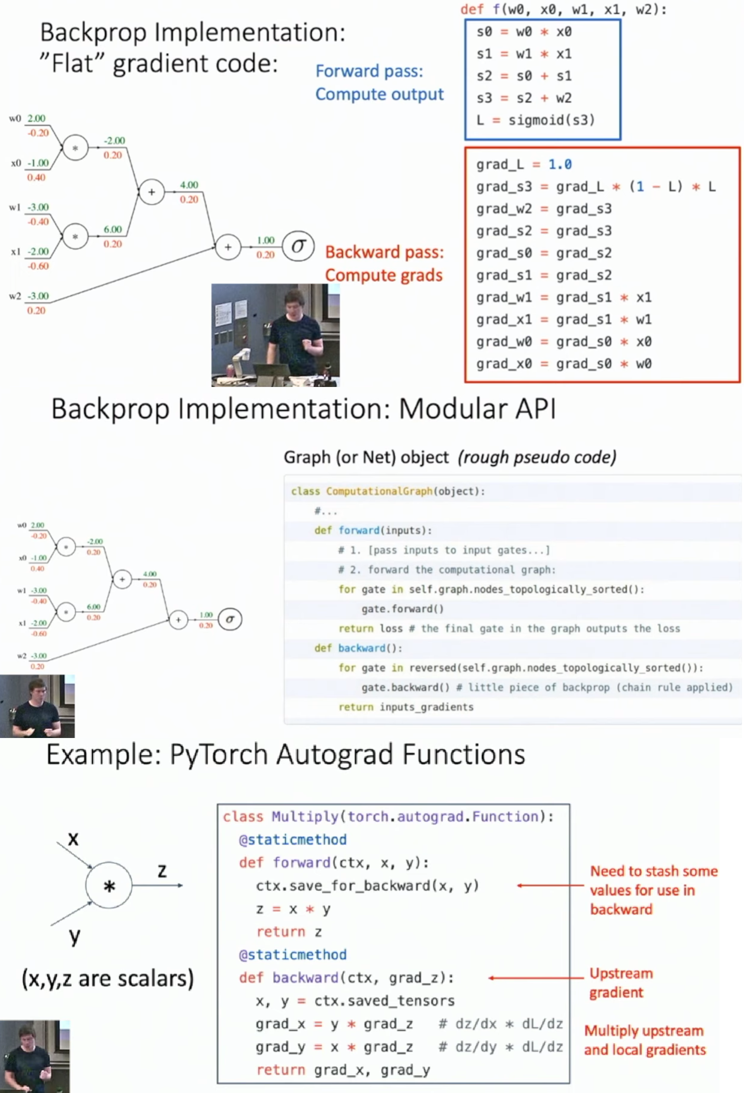
Backprop Implementation
- You can define your own node object in computation graph using pytorch API
Backprop with Vectors
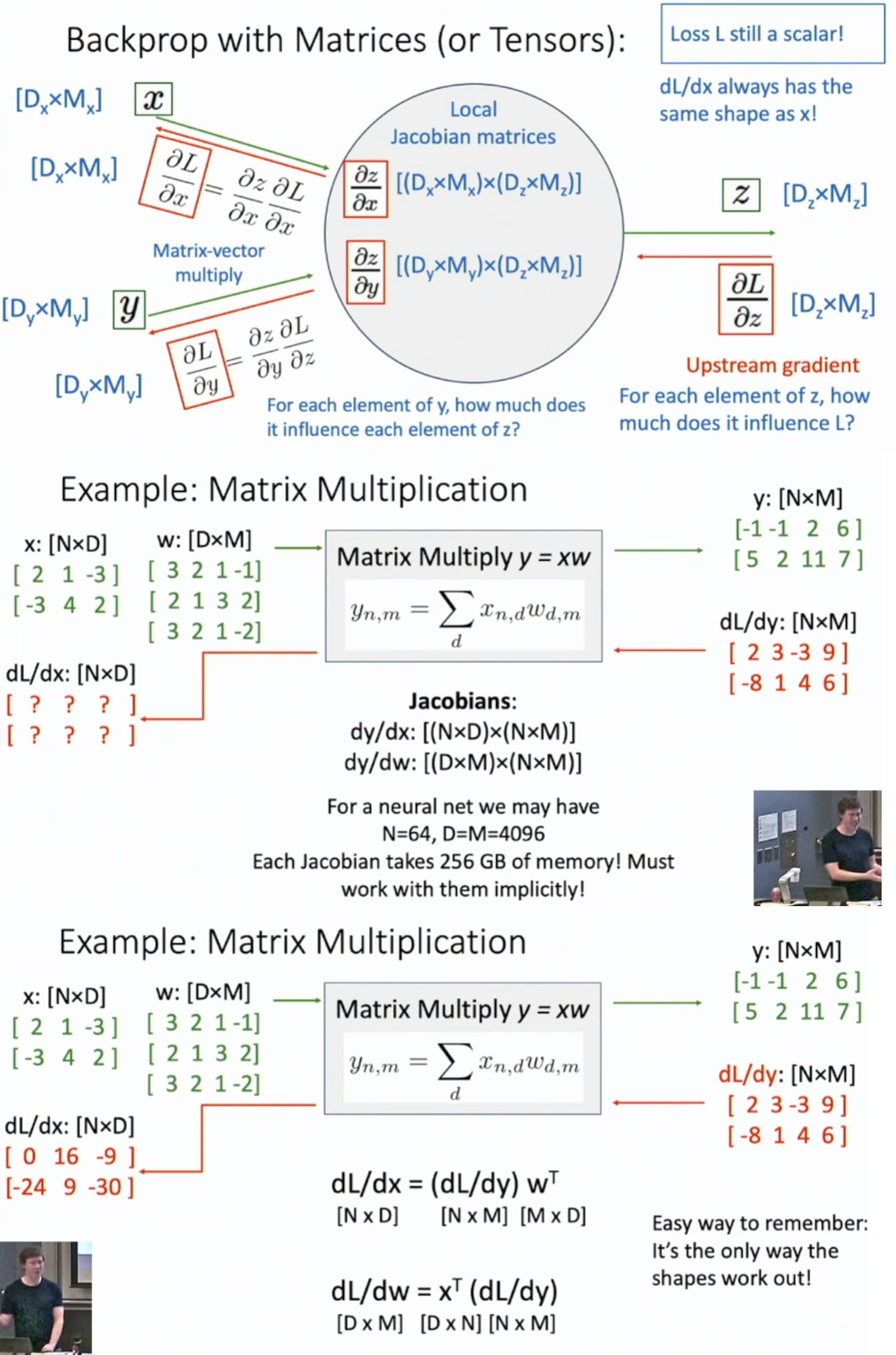
Backprop with Matrics
- \(dL/dx\) must have the same shape as \(x\) since loss \(L\) is a scalar
Assume we want to derive \(dL/dx_{i,j}\)
- Note that only the \(ith\) row of \(y\) is formed by \(x_{i,j}\) and corresponding coefficients are the \(jth\) row of \(w\).
- So \(dL/dx_{i,j}\) is just the inner product of the \(ith\) row of \(dL/dy\) and the \(jth\) column of \(w^{T}\), which leads to the result of \(dL/dx=(dL/dy)w^{T}\)
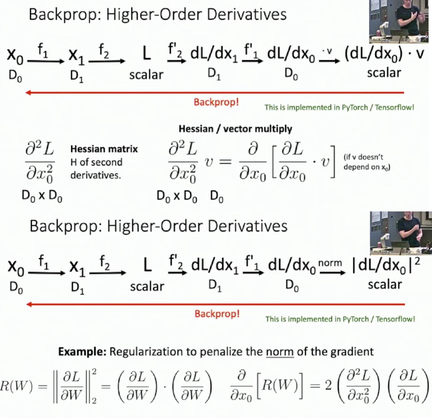
High-Order Derivatives
\(\frac{\partial ^{2}L}{\partial x_{0}^{2}}\) is \(D_{0} \times D_{0}\) dimension for it's the derivative of \(\frac{\partial L}{\partial x_{0}}\), which is a \(D_{0}\) dimension vector.
